On Typical Flaws of the Transformer Models for Inrush Current Evaluation
Sergey Zirka
Oles Honchar Dnipro National University, Dnipro
Yuriy Moroz
Oles Honchar Dnipro National University, Dnipro
1 Introduction
For many decades, the main, if not the only, equivalent circuit of a single-phase transformer was its T-model, Fig. 1. To avoid ambiguity and take into account the topology of the core and windings, we will use the terms inner and outer windings, instead of the primary and secondary windings. So, inductances LS1 and L′S2 are the so-called “leakage inductances” of the inner and outer windings, respectively, r1 and r′2 are their resistances. In order to reproduce hysteretic (quasi-static) properties of the core material and to account for the dynamic core losses and saturation, the magnetizing branch Lm in Fig. 1 is represented by an ATP-inductor DHM [1], which implements, starting with 2019 version, a Dynamic Hysteresis Model (DHM) [2].
Figure 1 – A conventional equivalent circuit of a single-phase transformer
Although the T-model does not “disclose the actual distribution of magnetic fluxes” within the transformer [3], it is widely used to describe its operation under the normal conditions and is a dominant transformer model in textbooks and papers.
Shortcomings of the T-model are revealed when the transformer core approaches saturation. Examples include inrush current and ferroresonance events, transformer operations under geomagnetically induced currents and those occurring in generator transformers during an out-of-phase synchronization. Each of these operations has its own characteristics and is considered separately. In this paper, we confine ourselves to considering inrush currents, which remain a subject of ongoing publications. Unfortunately, a lot of these papers focus on secondary details, mostly on hysteresis modeling [4], [5] and miss the fact that using the T-model in the inrush current evaluation is fraught with serious flaws.
The same can be said about the models of three-phase transformers [6], [7], [8], which neglect the recommendation in [9] that each wound limb must be shunted by an air branch (the latter divides the iron branches into legs and yokes).
The first disadvantage of the T-model is the artificial subdivision of the leakage transformer inductance LS (= LS1 + L′S2) into individual (physically non-existing) “leakage inductances” of individual windings. As will be shown in Section 2, such a subdivision can lead to underestimated inrush current peaks calculated for the inner winding and to overestimated current peaks for the outer winding.
In the shell and core type transformers (their legs and yokes are saturated differently), these errors are masked by another inherent drawback of the T-model, namely by the fact it contains only a single magnetization branch. To circumvent this masking effect and to better explain the errors due to the leakage subdivision, a toroidal core transformer is first considered in Section 2. Section 3 explains the necessity of introducing an additional magnetizing branch, which converts the T-model into a π-type structure devoid of the mentioned disadvantages.
Although this paper is devoted to generalized transformer models, simple analytical estimates of inrush current peaks are provided in Section 3 to facilitate subsequent explanations.
2 Toroidal transformer model
Our intention in this section is to show the errors in inrush current predictions due to the “leakage subdivision”. To avoid the problem of different magnetization levels of the leg and yokes, consider a transformer with a single magnetization branch, that is, a long toroidal core with two infinitely thin windings wound tightly over the entire core. The absence of the yokes and a large length l of the core allow one to straighten it out mentally into a ferromagnetic saturable rod, Fig. 2, whose ends are joined by a magnetic closure having an infinitely large magnetic permeability (µ = ∞).
Figure 2 – Toroidal transformer “unwrapped” into a straight wound rod
Neglecting the winding resistance and assuming an idealized voltage source, , switched to the inner or outer winding (each having N turns), the inrush current peak Im in the device of Fig. 2 can be calculated fairly accurately using inductance Lsat of the completely saturated wound core [10], [11], [12]:
where
Here, A is the cross section of the core steel, B0 is its initial flux density; BS (= 2.0 ‒ 2.03 T) is the saturation flux density of grain-oriented steel; h and deqv are the height and mean diameter of the excited winding.
It should be recalled that the leakage inductance LS is determined by the width d12 of the leakage channel between the inner winding 1 and the outer winding 2.
When the excited coil is the inner winding 1 (when deqv = D1), the open-circuit outer winding 2 “does not exist” [13] and the leakage channel does not participate in the magnetization process. This means that inductance LS is not involved in the inrush current evaluation and no part of LS can be included in the current path between terminals 1 and 0 of the inner winding in Fig. 3. However, a necessary element of the magnetization branch is inductance L01 which represents the insulation clearance d01 between the inner winding 1 and the grounded core.
Figure 3 – An equivalent circuit of a toroidal transformer
When the excited coil is the outer winding 2, i.e. deqv = D2, the space between winding 2 and the core includes the leakage channel (of width d12) and the innermost clearance (of width d01). Therefore, the inrush current path between terminals 2 and 0 in Fig. 3 should include the whole inductance LS plus the just mentioned inductance L01.
It should be clear that moving any part of inductance LS into the loop of the inner winding 1, that is, returning to the model in Fig. 1 would result in underestimation of the true current peak in the inner winding 1 and, respectively, in overestimation of the current peak in the outer winding 2.
For the toroidal transformer considered in this section, the Γ-type model in Fig. 3 is equally suitable for inrush current evaluation and modeling the rated operation. This is because the core length l used in the core loss evaluation is equal to the winding height h employed in (2). Quite different situation takes place in transformers with legs and yokes considered in the next section.
3 The Core and Shell Type Transformers
It is crucial to note that the core length l employed at the transformer design stage (it is used for the core loss evaluation) is several times greater than the height h of the winding used in the inrush current prediction. This makes inductance Lm in the general purpose models of Figs. 1 and 3 appreciably smaller than inductance Lsat in (2). Therefore, these models would always overestimate the inrush current significantly regardless of which winding is energized. The reason can be explained by different saturation depths of the wound leg and yokes.
Figure 4 – Main magnetic flux paths in a shell-type transformer with two concentric windings
When a transformer is energized, the core leg can reach very deep saturation. In this case, the magnetic flux density in the wound leg and the adjacent air channel(s) can reach values of the order of 3 T and higher. This is due to the fact that most of the leg is in a “tube” formed by the magnetizing winding. Regardless of the degree of saturation of the leg, no or a small part of its flux can escape from the tube.
The saturation of the side branches (SBs) of the core (they compose of the lateral limbs and the related yokes) remain moderate in the sense that the flux density in the SBs does not usually exceed 2 T. This is due to the fact that, as the SBs saturate, the magnetic permeability of their material approaches the vacuum permeability (µ0), resulting in arising shunting magnetic fluxes, designated as Ф0 in Fig. 4. The lengths of these air paths are shorter than that of the saturated SBs. Thus, the shunting fluxes Ф0 keeps the SBs from further saturation. Regarding the space occupied by Ф0, it depends on the winding which is energized. When the exited winding is the inner one, the flux in the leakage channel flows downward and merges with the flux flowing beyond the windings. When exiting the outer winding, the flux in the leakage channel flows upward and merges with flux Φ01.
These flux paths are reflected in the magnetic network in Fig. 5 [12] where F1 and F2 are sources of magneto-motive force of the inner and outer windings, respectively. The shaded elements represent hysteretic reluctances of the leg (ℜleg) and side branches (ℜSB), whereas unshaded elements designate linear reluctances of the paths in air (the subscripts of the ℜ01, ℜ12 and ℜ0 are the same as those of the magnetic fluxes).
Figure 5 – Magnetic equivalent networks of a two-winding transformer
Using the duality transformation [14], [15], the magnetic network in Fig. 5 is converted into its electrical equivalent shown between points 1 and 2 in Fig. 6.
Figure 6 – π-shaped electric equivalent circuit of a two-winding transformer
In deep saturation, the final slope dB/dH of B–H curve of any material from the DHM library is equal to the magnetic constant µ0 = 4π×10−7 H/m. It is important that the segment with slope µ0 lies at the level of the technical saturation of transformer steel (near 2 T), but not at 1.7-1.8 T sometimes taken carelessly. Therefore, the model behavior in saturation is determined by inductances L01 and L0. Their proper choice makes the model reversible, that is, capable of replicating inrush currents measured on terminals of both the windings.
At this point one should be cautious about uncritical use of π-models with equal magnetizing inductances of the leg and yoke branches. (This model version is suggested for the case of insufficient information about transformer design [16]). This simplification, as well as the absence of inductances L01 and L0, makes the π-model symmetrical that contradicts different magnetization curves for the leg and yoke in saturation first observed in [17] and then reprinted in Fig. 6.16 of [18].
The difference between two magnetizing branches at large flux linkages results in different magnetization curves and inrush current values determined for terminals of the whole transformer. Such curves calculated for the transformer in [12] are shown in Fig. 7 where flux linkages Ψ1 and Ψ2 are integrals of the voltages at points 1 and 2 of the model in Fig. 6.
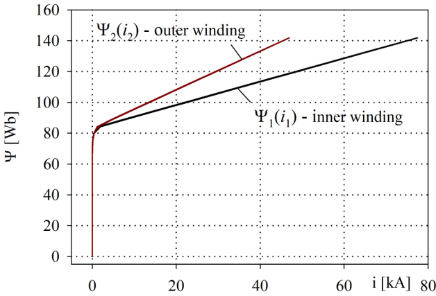
Figure 7 – Magnetization curves calculated from terminals of inner and outer windings
In their saturation regions, the Ψ–i curves in Fig. 7 can be characterized by differential inductances, Lsat1 = dΨ1/di and Lsat2 = dΨ2/di. The methods of their measurements are proposed in [19], [20] and [21] where inequality Lsat2 > Lsat1 was clearly demonstrated.
To account for the winding thicknesses, the model in Fig. 6 is provided by two groups of three inductances as shown in Fig. 8. This technique was proposed in [22] and then used in [23], [24] where inductances Lp are shown to be proportional to one sixth of the thickness of the corresponding winding.
When introducing inductances Lp, the values of L01 and L0 of the model are recalculated so as to maintain the reversibility of the model. This keeps unchanged the magnetization curves in Fig. 7 and thus inrush currents.
In concluding the paper, we can evaluate the influence of the hysteresis properties of the core material on the transformer behavior during inrush current events. For definiteness, the transformer is demagnetized thoroughly before each energization. Fig. 9 shows inrush currents calculated with the models in Fig. 6 and 8 excited from the inner and outer windings (assuming opposite winding open-circuited).
Figure 8 – π-equivalent circuit of a two-winding transformer, which accounts for the winding thicknesses
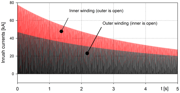
Figure 9 – Inrush currents on terminal of the inner and outer windings
It was found with certainty that both the current peaks in Fig. 9 and the rate of their decay practically do not depend on the hysteresis properties of the core and on the core loss at all. This is consistent with conclusions made in the recent modeling of ferroresonance processes in small voltage transformers [25] and in studying effects of geomagnetically induced currents in large 400 MVA units [26]. At the same time, accounting for material saturation is found necessary in all of these cases. For this reason, the saturation curve is included in all materials contained in the DHM library.
4 Conclusion
We have attracted attention to typical mistakes made in modeling transformer inrush currents. It is explained that the main mistake is the use of the convenient T-model and their three-phase derivatives. Their disadvantages are rooted in using separate leakage models of primary and secondary circuits, as well as in inability to reproduce different magnetization levels of the legs and yoke. We show the benefits of the π-model, but at the same time, caution against its oversimplification. Although we use an advanced hysteresis model to describe processes in the legs and yokes, it is shown that accounting hysteresis and core losses is completely optional in modeling inrush currents. These model properties have no visible impact neither on the current peaks nor their decay in time.
References
- H.Kr. Høidalen, L. Prikler, F. Peñaloza, ATPDraw, version 7.0 for Windows, User’s Manual, 2019.
- S. E. Zirka, Y. I. Moroz, N. Chiesa, R. G. Harrison, and H. Kr. Hoidalen, “Implementation of inverse hysteresis model into EMTP – Part II: Dynamic model,” IEEE Trans. Power Del., vol. 30, no. 5, pp. 2233-3241, Oct. 2015. doi: 10.1109/TPWRD.2015.2416199.
- A. Boyajian, Impedance characteristics of transformers. Ch. IV in Transformer Engineering L.F. Blume, G. Camilli, A. Boyajian, V.M. Montsinger, N.Y. John Wiley & Sons, 1938.
- H. Altun, S. Sünter,·Ö. Aydoğmuş, “Modeling and analysis of a single-phase core-type transformer under inrush current and nonlinear load conditions,” Electrical Engineering. doi: 10.1007/s00202-021-01283-9.
- A. Tokić, I. Uglešić, and G. Štumberger, “Simulations of transformer inrush current by using BDF-based numerical methods,” Hindawi Publishing Corp., Math. Problems in Eng., vol. 2013, Article ID 215647. http://dx.doi.org/10.1155/2013/215647.
- J. Pedra, L. Sainz, F. Córcoles, R. Lopez, and M. Salichs, “PSPICE computer model of a nonlinear three-phase three-legged transformer,” IEEE Trans. Power Del., vol. 19, no. 1, Jan. 2004. pp. 200-207. doi: 10.1109/TPWRD.2003.820224.
- A. D. Theocharis, J. Milias-Argitis, and T. Zacharias, “Three-phase transformer model including magnetic hysteresis and eddy currents effects,” IEEE Trans. Power Del., vol. 24, no. 3, pp. 1284–1294, Jul. 2009. doi: 10.1109/TPWRD.2009.2022671.
- P. S. Moses, M. A. S. Masoum, and H. A. Toliyat, “Dynamic modeling of three-phase asymmetric power transformers with magnetic hysteresis: No-load and inrush conditions,” IEEE Trans. Energy Convers., vol. 25, no. 4, pp. 1040–1047, Dec. 2010. doi: 10.1109/TEC.2010.2065231.
- C. M. Arturi, “Transient simulation of a three-phase five-limb step-up transformer following an out-of-phase synchronization,” IEEE Trans. Power Del., vol. 6, no. 1, pp. 196–207, Jan. 1991. doi: 10.1109/61.103738.
- N. Chiesa, B. A. Mork, H. K. Høidalen, “Transformer model for inrush current calculations: Simulations, measurements and sensitivity analysis,” IEEE Trans. Power Del., vol. 25, no. 4, 2010, pp. 2599–2608. doi: 10.1109/TPWRD.2010.2045518.
- S. V. Kulkarni and S. A. Khaparde, Transformer Engineering: Design and Practice. New York: Marcel Dekker, 2004.
- S. E. Zirka, Y. I. Moroz, C. M. Arturi, N. Chiesa, and H. K. Høidalen, “Topology-correct reversible transformer model,” IEEE Trans. Power Del., vol. 27, no. 4, pp. 2037–2045, Oct. 2012. doi: 10.1109/TPWRD.2012.2205275.
- S. Jazebi, F. de Leon, N. Wu. “Enhanced analytical method for the calculation of the maximum inrush currents of single-phase power transformers,” IEEE Trans. Power Del., vol. 30, no. 6, pp. 2590–2599, Dec. 2015. doi: 10.1109/TPWRD.2015.2443560.
- E. C. Cherry, “The duality between interlinked electric and magnetic circuits and the formation of transformer equivalent circuits,” Proc. Phys. Soc. B 62. pp. 101–111, 1949. doi: 10.1088/0370-1301/62/2/303.
- S. Jazebi, S. E. Zirka, M. Lambert, A. Rezaei-Zare, et al., “Duality derived transformer models for low-frequency electromagnetic transients—Part I: Topological models,” IEEE Trans. Power Del., vol. 31, no. 5, pp. 2410-2419, 2016. doi: 10.1109/TPWRD.2016.2517327.
- F. de León, P. Gómez, J. A. Martinez-Velasco, and M. Rioual, “Transformers,” Chapter 4 in Power System Transients. Parameter Determination, J. A. Martinez-Velasco (ed.), CRC Press, 2009.
- M. Kh. Zikherman, “Magnetization characteristics of large transformers,” Elektrichestvo, no. 3, pp. 79-82, 1972. [in Russian].
- H.W. Dommel, Electromagnetic transients program reference manual (EMTP Theory Book); Bonneville Power Administration, Portland, OR, USA, 1986.
- S. Calabro, F. Coppadoro and S. Crepaz, “The measurement of the magnetization characteristics of large power transformers and reactors through DC excitation”, IEEE Trans. Power Del., vol. 1, no. 4, pp. 224-232, Oct. 1986. doi: 10.1109/TPWRD.1986.4308052.
- S. Jazebi, F. de León, A. Farazmand, and D. Deswal, “Dual reversible transformer model for the calculation of low-frequency transients,” IEEE Trans. Power Del., vol. 28, no. 4, pp. 2509-2517, Oct. 2013. doi: 10.1109/TPWRD.2013.2268857.
- W. Sima, B. Zou, M. Yang, F. de León, “New method to measure deep-saturated magnetizing inductances for dual reversible models of single-phase two-winding transformers,” IEEE Trans. Power Del., vol. 36, no. 1, pp. 488-491, Feb. 2021. doi: 10.1109/TEC.2020.3023596.
- H. Edelmann, “Descriptive determination of transformer equivalent circuits,” Archiv für elektrische Übertragung, vol. 13, no. 6, pp. 253-261, 1959. [in German].
- S. E. Zirka, Y. I. Moroz, C. M. Arturi, “Accounting for the influence of the tank walls in the zero-sequence topological model of a three-phase, three-limb transformer,” IEEE Trans Power Del., vol. 29, no. 5, pp. 2172–2179, Oct. 2014. doi: 10.1109/TPWRD.2014.2307117.
- J. Zhao, S. E. Zirka, Y. I. Moroz, C. M. Arturi, “Structure and properties of the hybrid and topological transformer models,” Int. J. Electr. Power & Energy Systems, vol. 118, 2020, 105785. doi: 10.1016/j.ijepes.2019.105785.
- S. E. Zirka, Y. I. Moroz, A. V. Zhuykov, D. A. Matveev, et al., “Eliminating VT uncertainties in modeling ferroresonance phenomena caused by single phase-to-ground faults in isolated neutral network,” Int. J. Electr. Power & Energy Systems, 2021, vol. 133. Paper 107275. doi.org/10.1016/j.ijepes.2021.107275.
- S. E. Zirka, Y. I. Moroz, J. Elovaara, M. Lahtinen, et al., “Simplified models of three-phase, five-limb transformer for studying GIC effects,” Int. J. Electr. Power & Energy Systems, vol. 103, pp. 168-175, 2018. https://doi.org/10.1016/j.ijepes.2018.05.035.